THE GREAT SMOG: WHEN LONDON COULD NOT BREATHE
How coal smoke and a temperature inversion created London’s five-day smog, why death estimates differ and what the 1956 Clean Air Act changed.
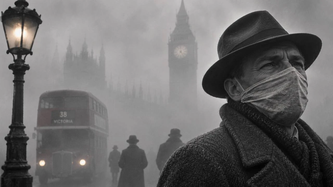
Editorial illustration supplied for PRESDA.
From December 5 to 9, 1952, a dense, smoke-laden fog lay over London. Cold conditions increased demand for coal fires, and a layer of warmer air held pollution close to the ground. Smoke from homes, power stations and industry mixed with fog and accumulated where people lived and travelled. The haze changed how the city worked over five days. Its effects on health lasted longer. A contemporary estimate of the immediate toll and a later study of the following months describe different parts of the same disaster. UK Met Office Great Smog case study London Museum account and archive Greater London Authority analysis Bell and Davis mortality reassessment
Why the smoke stayed near the ground
| Event or period | Recorded finding |
|---|---|
| 5–9 December 1952 | Dense smoke-laden fog covers London |
| December 1952 | About 4,000 excess deaths in the estimate cited by London City Hall |
| December 1952 to February 1953 | About 12,000 excess deaths in a later research estimate |
| 1956 | Clean Air Act introduces powers for smoke control areas |
Under conditions that allow mixing, polluted air near the ground can be carried away or diluted as it rises. In a temperature inversion, air above a cooler surface layer is warmer. That arrangement restricts vertical mixing. The Met Office describes high pressure, light winds and a temperature inversion as key conditions in December 1952. Meanwhile, households burned coal to keep warm and industrial and power sources continued to emit pollution. The weather affected where the emissions went and how long they remained close to people. UK Met Office Great Smog case study Greater London Authority analysis
How fog became smog
Fog consists of tiny water droplets. Particles from combustion can serve as surfaces on which the droplets form. The droplets and particles scatter light and the air can contain gases and chemicals from the same pollution sources. A fog that limits visibility and a smog that exposes people to pollutants are related observations, but they do not measure the same thing. Two places with similarly poor visibility may have different mixtures of smoke, moisture and gases. London’s coal use made the quality of that trapped air unusually dangerous. UK Met Office Great Smog case study Greater London Authority analysis
What the city experienced over five days
The London Museum describes disruption to travel and everyday activity. People were accustomed to fog, yet the density and persistence of that week made it exceptional. A bus, car or pedestrian could have difficulty making out what was ahead. The same haze could reach indoor settings. Travel reports and photographs show what people could see and do. Hospital records and mortality records help reconstruct what that exposure did to health. The two kinds of evidence explain why a scene that looks like a transport story can also belong to public-health history. UK Met Office Great Smog case study London Museum account and archive
Why the smog became visible in death records
Medical and vital records allow researchers to look at deaths during and after the episode. Excess mortality means deaths above the number expected over a specified period. It is not a list of every death certificate on which the event was named. The result depends on what baseline is chosen, which period is counted and how other possible causes are handled. That is why it helps to attach an explicit time window to a number, even when the figure has been quoted many times. Greater London Authority analysis Bell and Davis mortality reassessment
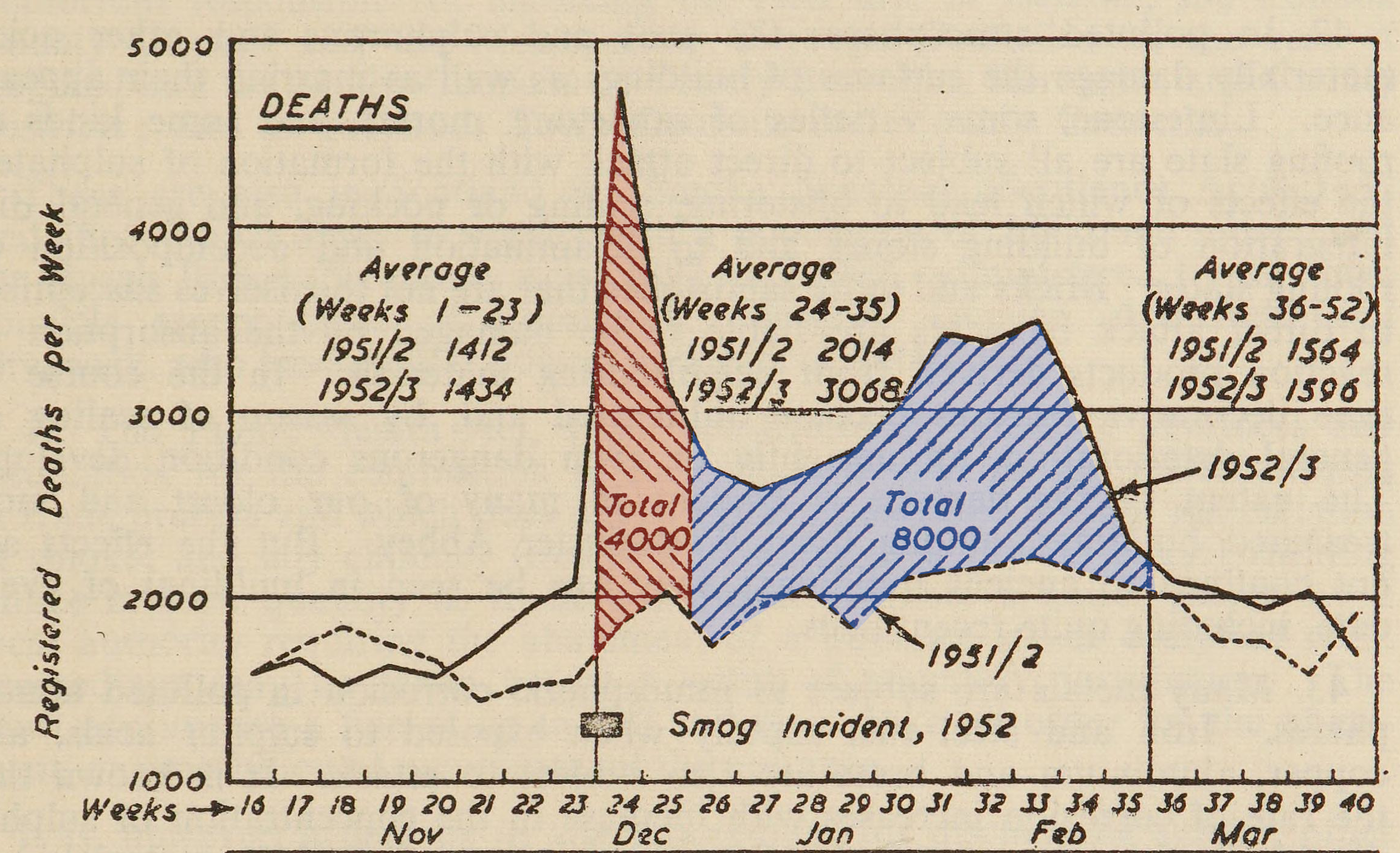
Chart from the 1953 UK air pollution inquiry showing the rise in deaths around the December 1952 smog.
UK Committee on Air Pollution, 1953 interim report / Wikimedia Commons · Public domain
Why sources cite about 4,000 and about 12,000
The Greater London Authority summarises an estimate of about 4,000 excess deaths during December 1952. A peer-reviewed reassessment by Michelle Bell and Devra Davis estimated about 12,000 excess deaths over the longer period from December 1952 through February 1953. The estimates are not separate groups to add together. The longer period includes December, and the later analysis used a different method to assess persistent effects. A comparison that gives the figures without the study and time period makes the apparent disagreement larger than it is. Greater London Authority analysis Bell and Davis mortality reassessment
What the longer window can show
People can experience health consequences after the visible pollution clears. Studying the weeks that follow allows researchers to test whether mortality remained above expected levels. Extending the window also makes the analysis harder, because other factors can affect health at the same time. The study’s method and assumptions matter more than the appearance of a larger total. The two figures show how a famous event can be measured as both a short period of exceptional weather and a longer period of elevated risk. UK Met Office Great Smog case study Greater London Authority analysis Bell and Davis mortality reassessment
What the 1956 Clean Air Act changed
Across London, the week raised a question that weather forecasting alone could not solve. The emissions came largely from identifiable sources that used fuel. The Clean Air Act 1956 as enacted provided for smoke control areas and included measures addressing smoke from furnaces and chimneys. It changed the tools available to local authorities. The law still had to be implemented through decisions about fuels, equipment and locations. A date on the Act does not imply that streets became smoke-free overnight, and the Met Office records subsequent efforts and the later 1968 Act. UK Met Office Great Smog case study London Museum account and archive Clean Air Act 1956 as enacted
What London’s change required from households
A smoke control rule changes what can be burned and can require different equipment. A policy aimed at emissions therefore reaches everyday decisions about how a room is heated and what a household can access. Citywide improvements also depend on changes in power generation and industry. A comparison of one winter with a later one has to account for weather as well as the change in fuel. For another example of how the source of domestic heat matters, read PRESDA’s account of Iceland’s geothermal networks. Greater London Authority analysis Clean Air Act 1956 as enacted
What survives in the evidence
The records preserve several versions of the same week. Weather observations show the conditions that kept emissions in place. A museum photograph can show how far a person could see in one street. Mortality studies describe deaths over stated periods, and legislation shows what powers were adopted later. None of those records alone can describe the whole event. Their combination explains why a few days of heavy fog became a lasting example of what happens when air pollution reaches a whole city under unfavourable weather. UK Met Office Great Smog case study London Museum account and archive Bell and Davis mortality reassessment Clean Air Act 1956 as enacted
Four different clocks for the same disaster
The dates of the weather event, the period of exposure, the weeks in which excess deaths occurred and the years it took to pass a law answer different questions. The fog lifted on December 9. Someone exposed during those five days could still die afterward, so a death tally cut off when visibility returned would miss some of the burden. London’s contemporary observers could compare death registrations and air measurements, while later researchers could examine a longer window and test explanations for the winter increase. Their totals should always be read with their dates attached. UK Met Office Great Smog case study London Museum account and archive Bell and Davis mortality reassessment
The legislation had its own timetable. Councils could designate smoke control areas, within which households could comply through approved fuels or installations. Converting a hearth, getting a supply of suitable fuel and establishing local rules were practical steps between passing the Act and reducing emissions. That distinction helps explain why the Act’s date marks a policy change while the air took longer to improve. Greater London Authority analysis Clean Air Act 1956 as enacted
How to read the archival mortality chart
The reproduced chart from the 1953 air-pollution inquiry compares weekly registered deaths in 1952–1953 with those in the previous year. Its vertical axis counts registered deaths per week, and its horizontal axis moves from November through February. Those are observations over a period, while attributing an excess to pollution requires an argument about what would otherwise have happened. The shaded annotations show how the author grouped differences after the smog. They should be read as the interpretation in that document. The later Bell and Davis study tests the longer aftermath through its own analysis. A similar-looking total in two sources does not mean they used the same method. The chart is valuable because it makes visible both the sharp initial peak and the need to examine subsequent weeks. Its source and publication date are therefore as important as the numbers drawn on it.
FAQ
Frequently Asked Questions
What caused the Great Smog of London?
Coal smoke accumulated near the ground under stagnant conditions and a temperature inversion, mixing with fog.
How many people died?
London City Hall cites about 4,000 excess deaths in December. A later study estimated about 12,000 over December through February.
What was the government response?
The 1956 Clean Air Act provided for smoke control areas and other emission controls.
PRESDA Dispatch
Stay Informed. Stay Aware.
A sharp briefing across AI, gaming, sport, business, world affairs, paparazzi, and lifestyle.